Linear Chain Model

This tutorial demonstrates running the Linear Chain Model at a temperature of 500 K for a simulation time of 50 ps and compare the simulation result obtained from SHARP Pack with the exact analytical result.

Follow the steps below:

Prepare param.in

Prepare input file param.in with the model and simulation parameters setting temperatrue  500.

#linear chain model input parameter
model        db2lchain
nParticle    20
nbeads       1
iseed        12345
ncore        1
tstep        10.0
nsteps       206700
ntraj        200
temperature  500.0
rsamp        gaussian
vsamp        gaussian
iprint       100
finish

Run Simulation

Run the simulation using one of the following methods:

# direct execution
$ ./sharp.x

# for running on a local machine
$ sh job-script-local.sh

#for submitting jobs on an HPC cluster (Slurm)
$ sh job-script-hpc.sh

Plot Result

Use gnuplot script plot-pop.gnu to plot the convergence of population to exact Boltzmann distribution.

#!/usr/bin/gnuplot
set encoding iso_8859_1
set key right center
set terminal pdf size 4in,2.8in enhanced color font 'Helvetica,16'
set border lw 2.5
set tics scale 1.2
set ylabel "{/Helvetica=22 Population}"
set xlabel "{/Helvetica=22 time (ps)}"
set mytics 2
set mxtics 2
set grid xtics ytics

e1=0;e2=8.0;
temp=500.0  #in Kevlin
kbT=0.0083*temp

#exact Boltzmann distribution
p1(x)=exp(-e1/kbT)/(exp(-e1/kbT)+exp(-e2/kbT));
p2(x)=exp(-e2/kbT)/(exp(-e1/kbT)+exp(-e2/kbT));

outfile = 'fig-population.pdf'
set output outfile
set key opaque samplen 1.0 spacing 1.3 font "Helvetica, 14"
plot 'pop_adiabat1.out' u (column(1)/41340):2 w l lc 3 t'FSSH: P_1',\
     'pop_adiabat1.out' u (column(1))/41340):3 w l lc 4 t'FSSH: P_2',\
      p1(x) w l lc 6 lw 5 t'Exact: P_1',\
      p2(x) w l lc 7 lw 5 t'Exact: P_2'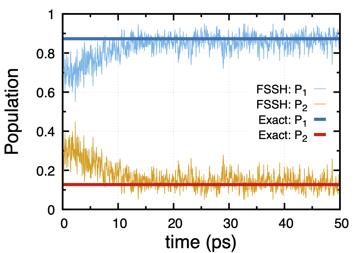

Fig. 4 Population convergence of linear chain model to exact Boltzmann distribution at 500 K by FSSH method.